We are a tutoring company. We have a certain amount of free tutoring to distribute in the amount of $12,000. I have a spreadsheet that creates contact cards for new students. I want to create a spreadsheet that will populate with new client names and their date of first sessions. I also want a column that will calculate how much we’re spending as we add new students, so I can look at this spreadsheet to see how many more slots we have for students. Each student costs $500. So that column would start with the 1st student and should say $11,500, 2nd student should say $11,000 and so on. When I type in a new profile card, the name of the student and their first session date should show up on the the spreadsheet and the last column will calculate how much money we have left. I should be able to refer to this sheet before registering new people to make sure we still have spots left.
Hi There!
There are a few ways you could go about this - if you would like a simple spreadsheet of students and assume all of the students in this list are part of the free tutoring, you could set it up like the page at the link below;
https://public.getgrist.com/vqkssfq82wRF/Private-Tutor-Billing-Community-538
At the top, you see a summary that shows number of students, total amount spent, amount remaining and # of slots available. Below that is the list of students and contact card to fill out their information.
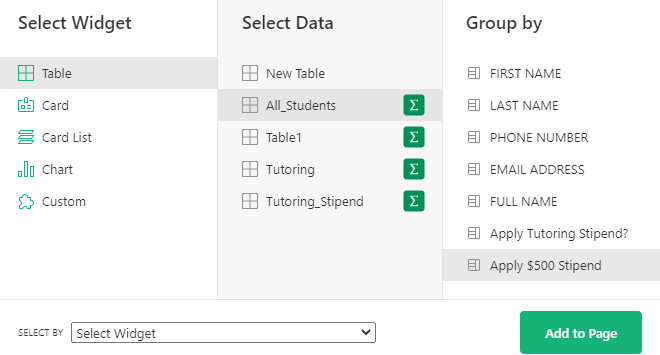
Now, if you want to keep this list of students well after the stipend ends, you could include a column to select if the tutoring stipend applies. You’ll see this in the All Students page at the link below. Only students who have the Apply Tutoring Stipend column checked are included in the stipend totals at the top.
https://public.getgrist.com/eDZwjE7QMMHD/Private-Tutor-Billing-Community-538-copy
You’ll see that there are also ‘Tutoring’ and ‘Tutoring Stipend’ pages - this would be the third option. You could have one page that includes All Students then just include the students where the free tutoring stipend applies in this separate table. The students included in this table are used to calculate the amount remaining on the Tutoring Stipend Page.
Let me know what you think of these options. If you want it set up a bit differently, let me know and we can make some changes!
Natalie, I’m so grateful! I haven’t had a chance to check this out in full but I’ll let you know. Thank you!!
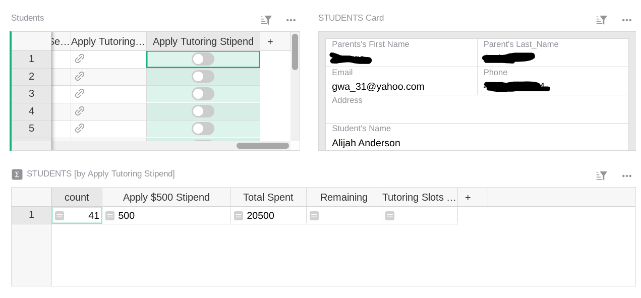
Hi! I like the second option. I already have a list of students set up and student cards. As you can see from my screenshot, I added a column that you can toggle on and off to apply tutoring stipend. The problem is that the spreadsheet adds ALL of the students. I need it to only include the students that have the Apply stipend option toggled on.
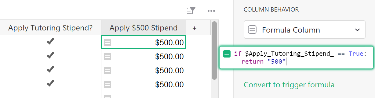
I had a column hidden in the Students table that applied the $500 stipend/student. I realize it’s not terribly helpful if you can’t see it!
After creating the ‘Apply Tutoring Stipend’ column, I created a column to calculate the cost. Since each student is $500, I have a formula that adds this $500 when ‘Apply Tutoring Stipend’ is marked as True.
if $Apply_Tutoring_Stipend_ == True:
  return "500"
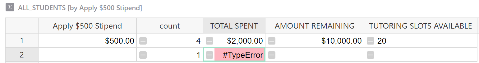
Then, create the summary table and summarize by ‘Apply $500 Stipend’ (the column with the formula, not the toggle). It will summarize how many students are counted. We’ll add the rest of the formula columns using the formulas below;
TOTAL SPENT
IFERROR($Apply_500_Stipend*$count, None)
AMOUNT REMAINING
IFERROR(12000-$TOTAL_SPENT, None)
TUTORING SLOTS AVAILABLE
IFERROR($AMOUNT_REMAINING/$Apply_500_Stipend, None)
We are using IFERROR to remove the errors that will appear on the count of students who do not have tutoring applied. If I remove this from the formula, you’ll get errors like you see below. No amount is applied for the students who have not received the stipend but it’s expecting to multiply two numbers where there is only one.
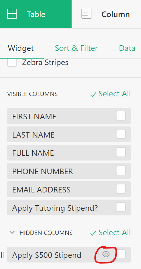
You can hide the ‘Apply $500 Stipend’ column in your table if you’d like. As long as you set the ‘Apply Tutoring Stipend?’ toggle to True/On, the formula will run and the $500 for that student will be applied. You can hide/unhide columns in the right-hand Table menu. Hover over the column name and an eye icon will appear. Click this to make a hidden column visible. If you want to hide a column, hover over the column name and then click the hide icon that appears.
I studied your sheet last night and figured it out. Finally saw the hidden column. It works now! Thanks so much for your help. I’m going to dig into your answer because I need to understand why the spreadsheet works! I don’t understand the formulas at all. 
I can walk through them for you and let you know what each is doing! Anything with $ ahead of it is a column name. Since the column names are long, it can seem overwhelming.
if $Apply_Tutoring_Stipend_ == True:
  return "500"
This is a handy Python function to know. You may run into versions of it throughout our many templates! Three key points to notice here -
-
To say equals, it is actually two equals signs, rather than one. I like to think about it as ‘I am so sure that this is equal that I’m going to put two equals signs’! Similar to when you’re excited and have multiple exclamation points. Also available comparisons: less than (<), greater than (>), less than or equal to (<=), greater than or equal to (>=) . If you’d like to see an example using some of these, check out the Stock Alert column in our Inventory Manager template.
-
True vs False: When a toggle column type is toggled off or unchecked, this means it is set to False. when a toggle column type is toggled on or checked, this means it is set to True. When you apply the tutoring stipend to a student by toggling the button, it sets it to True, meaning we are applying the stipend.
-
Be sure to indent the second line. To add a second line in a formula, click ‘shift’ + ‘return’. Then tab to indent.
if some statement satisfies some condition, return the given argument. In this case, it’s saying if the ‘Apply Tutoring Stipend’ column is equal to True (toggle on/checked), the value in this field should be ‘500’.
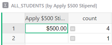
Moving into the summary table - when we created this table, we selected the Summation button and grouped by the ‘Apply $500 Stipend’ column (this is where the formula enters $500 when the other column is set to true).
It shows us the number of students who have $500 entered in this column and it shows us the number of students who have nothing entered in that column. That’s all done for us by selecting the summary table.
TOTAL SPENT
IFERROR($Apply_500_Stipend*$count, None)
If we take out the IFERROR portion of this, it’s much easier to see what is going on
$Apply_500_Stipend*$count
Here, we have a simple math equation multiplying two values from two columns. We are multiplying the value in the ‘Apply $500 Stipend’ column times the number of students who are marked to receive it in order to find the total amount spent. The count column was auto-calculated for us when we created the summary table. This number is always up-to-date as it’s constantly checking for updates.
Going back to the full equation -
IFERROR($Apply_500_Stipend*$count, None)
IFERROR follows this format -
IFERROR(value, value_if_error)
It’ll return the first value if there is no error, otherwise returns the second argument. In our case, if there is no error, it multiplies the two columns together. If there is an error, it returns None which we see as an empty field.
AMOUNT REMAINING
IFERROR(12000-$TOTAL_SPENT, None)
Again, removing the IFERROR portion of the formula, we get the following;
12000-$TOTAL_SPENT
12000 is the total amount available for the stipend minus the value we just calculated in the equation above for the Total Spent column to get the amount remaining.
TUTORING SLOTS AVAILABLE
IFERROR($AMOUNT_REMAINING/$Apply_500_Stipend, None)
Removing the error portion of the formula;
$AMOUNT_REMAINING/$Apply_500_Stipend
Dividing the Amount Remaining (calculated above) by the value in the ‘Apply $500 stipend’ column (which is $500) to get the number of available slots.
I hope this helps!