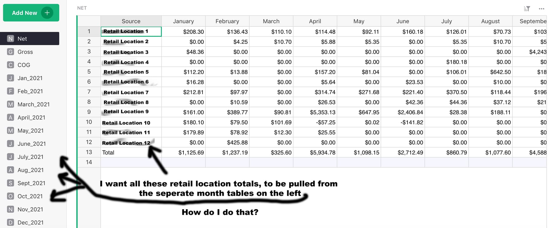
Hi I really like Grist, but I’m having difficulty figuring out something that is probably really simple. I’m sure their are multiple ways of creating this document, but I uploaded the information that I currently had in an Excel document. I’m an artist and sell at different locations, and created a table for each month with all the retail locations. I have a formula to calculate the Net and Gross profit for each of these locations in a given month. I also created a widget table for the monthly sum of each location in that month. I want to pull the sum from each location in each month to auto calculate my Net and Gross total on a new table like the image shown. How do I do that?
Hi Eric! Welcome to the Community.
I made a quick example for you. Check it out at the link below:
https://public.getgrist.com/vSUAM9o9TpuQ/Community-668/p/1/m/fork
I made a few guesses on how each month was set up - let me know if I am way off and I can rewrite formulas based on your actual setup.
We are using our lookupOne formula. The general format for this formula is:
[Table_Name].lookupOne([A]=$[B]).[C]
[Table_Name] is the name of the table you want to lookup data in. [A] is the column in the table being looked up (named at the beginning of the formula), [B] is the column in the current table / the table you are entering the formula in and [C] is the data you want for that record.
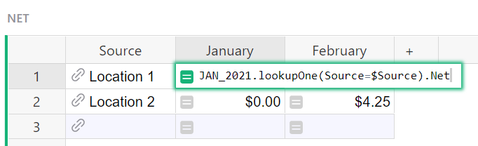
The formula you see here checks the JAN_2021 table for a record where the Source matches the Source in this table (Location 1). If it finds a record, it pulls the data from the Net column. For the February column, you would change table name to FEB_2021. Or if you’re on the Gross table, you’d just change Net to Gross to pull in data from the Gross column of the specified table.
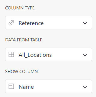
If you don’t already have your locations as References, I would recommend it. This would ensure that they are spelled correctly in each table so all calculations would work as expected. To do this, just create a new table. List out all Locations. Then, in each table, turn your Source column into a reference type column that pulls data from the Name column of this new table. Assuming they are all spelled correctly, they’ll automatically match up. In the future, you can select your location from the dropdown!
Let me know if you have any questions!
Thank you for the quick reply and amazing answer. I think this will work. I was trying to make a reference list and it kept giving me an error. I really appreciate you helping me out.
1 Like
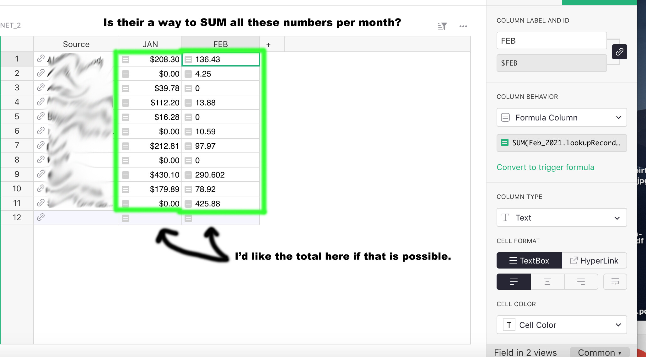
Okay I tried, but I keep getting an error message. I attached a screen shot of how my JAN_2021 is set up and I have a widget with the SUM for each retail location. I want that total SUM on the bottom widget for each location pulled over to the new table, but it doesn’t want to. I also attached a screen shot of the error message.

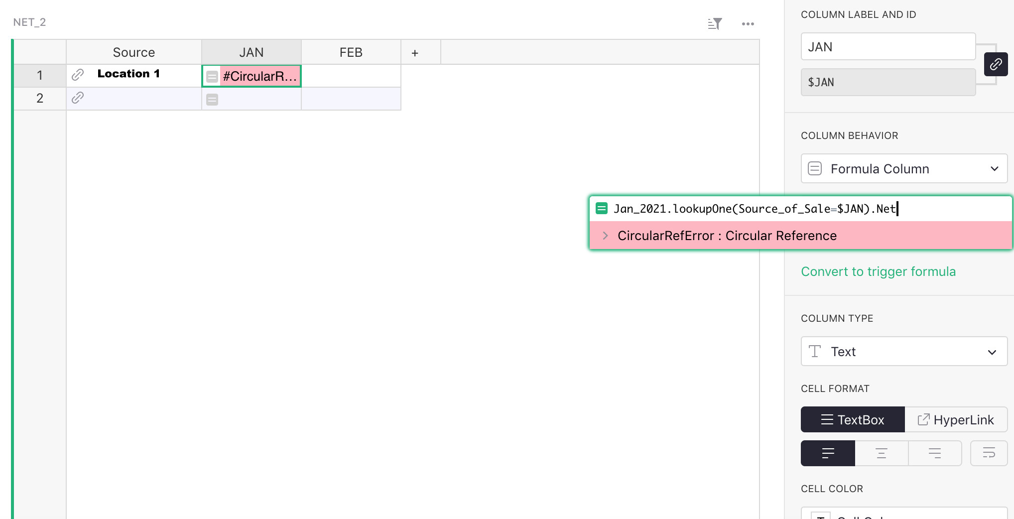
Thanks for sharing the screenshot - I have a new formula for you below. The error you are seeing (#CircularReference) is because the Column JAN is being called in the formula for itself. In the formula, it would be (Source_of_Sale=$Source) because you want the two locations to match.
New formula to get the sum
SUM(Jan_2021.lookupRecords(Source_of_Sale=$Source).Net)
This is what your summary table is doing. We can’t use summary tables in formulas so we are using this formula to get the same result.
The difference here is that we are using SUM() and lookupRecords. Before, we used lookupOne which only finds us one result where the sources match. Since there are multiple, we use lookupRecords so it finds all records in the Jan_2021 table where Source of Sale and Source match. Then, it finds the Net for each record and sums it all together!
For the Gross table, the formula would be
SUM(Jan_2021.lookupRecords(Source_of_Sale=$Source).Gross)
1 Like
YES! That worked! Thank you so much. This software is really neat, and is way more visually easy on the eyes.
1 Like
Hey Natalie,
If you could please help me with one other thing. How can I get it to populate the total per column at the bottom of each month?
Hi Eric,
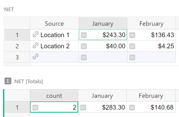
Because formulas affect the entire column, it’s not possible to add the total in the bottom row. You can add a summary table that sits just below this table and have the totals in line with the amounts that way. Select the green Add New button and add a new widget to the page. Select Widget = Table, Select Data = Net then click the green summation button. This will sum all numeric columns. Then click apply.

Then, you’ll have the totals for each column. This will update every time you add a new row.
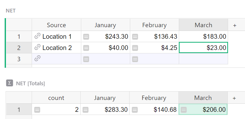
If you add a column, you can either delete and re-add the widget or copy/paste the formula from the prior month total to a new column and change the month name. For example, the formula for February is:
SUM($group.February)
If you add a March column to the Net table, you would add a new column to the Net [Totals] table with:
SUM($group.March)
1 Like
This is perfect. Thanks again!
1 Like
Hi. I have a similar setup but want to total across the columns, so in Eric’s example, a total for all months for Location 1
I tried adding a Widget but could not get it to sum as I want.
Any other suggestions please? Thanks!
P.S. It would be really useful for beginners to be able to see examples of all the Functions shown here: Function reference - Grist Help Center
Hello,
You might add a Total column in NET [Totals], with the formula:
SUM($January,$February,$March)
Thanks for your help but SUM only allows 2 entries:
e.g. SUM($January,$February)
The solution I used was to take it back into Google Sheets ![]()
I also considered turning the data round with months in the first column but couldn’t figure out how to do that either from the raw data I have.
SUM supports multiple entries:
I think you mix sum (Python built-in) and SUM (from Grist). SUM(1,2,3) works and gives 6.
Thanks guys, that did the trick! ![]()