In Grist this is called a recursive formula. It looks up the previous row, and then just compares earnings (see documentation).
Edit to add working with date column:
Ah, in Interests_P2P the date column is an actual date, rather than a number, so this is more like the example in the documentation for recursive functions. You can find the previous date with:
Ah, in Interests_P2P the date column is an actual date, rather than a number, so this is more like the example in the documentation for recursive functions. You can find the previous date with:
Thank you, Paul, for your help - I really appreciate it!
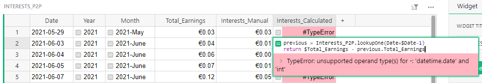
Your formula works except for consecutive entries. I’ve updated my example - check row #6.
The interests here should be €0.12 - the formula takes the value from the previous day, but since that value is zero, because I have no entry for the 2021-06-13, it returns €0.24. Which is wrong.
Is it possible to calculate the lookup based on the row-index?
If you can have gaps in the sequence, there is a general purpose method you can fall back on. Bear with me, it takes a little explaining
First, add an extra table to your document, call it for example Order. Then rename a column to be for example Interests_P2P (the name isn’t important, just adds clarity). Then, add a single row and set this formula for the column:
This means “calculate a list of record ids of the Interests_P2P table, ordered manually (by order of creation, and then any dragging around of rows in UI to reorder them)”. Alternatively you could sort by 'Date' or any other column name. The sort order you choose defines what you mean by a previous row/record.
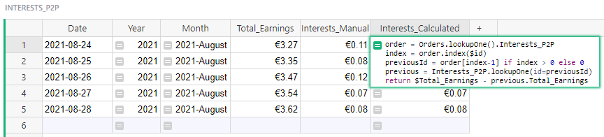
Now we can go back to Interests_Calculated and tweak the formula there to use the ordering we created:
order = Order.lookupOne().Interests_P2P
index = order.index($id)
previousId = order[index-1] if index > 0 else 0
previous = Interests_P2P.lookupOne(id=previousId)
return $Total_Earnings - previous.Total_Earnings
In summary this:
Gets the order we calculated in the Order table
Finds where the current record is in this order
Finds the id of the record just before that (being a little careful about the very first one)
Uses that id to look up the previous record
Then calculates difference as before
I’ve updated my example (by the way, to share yours, you’d need to turn on public access, otherwise your document is kept private).
If this all seems a lot of work for a common task: you’re not wrong! This is where the “database” side of Grist shows itself a bit - there are no natural row numbers in databases. There are row ids, and Grist has an $id available for every record row, and those ids are almost sequential - except if you delete or manually reorder rows.
We do have a plan to wrap the general method in this example up into something user friendly, but hopefully it’ll do the job for you - and thanks for persisting in your feedback @Haidosu !
Good morning @paul-grist, thank you for your answer!
This provides the solution in the example document!
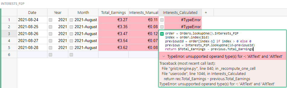
I tried to recreate the minimalistic example from my public document within my non-public document.
Here I copy-pasted some rows from it and get another error:
Since the columns Total_Earnings and Interests_Manual are highlighted I assume that something went wrong within that procedure, because after manually retyping the copied values, each highlighted cell went back to white background. After finishing the last cell, the formular worked like a charm as shown below. This could be a point of interest for you.
I have an assumption here:
Create a new column without changing the column type to currency.
Now, copy-paste values from a currency column and then change the column type to currency.
The copied values are now highlighted red.
You have to re-copy-paste them to be correctly interpreted.
Hope this information is helpful for you!
Could you consider implementing automated content type detection? @paul-grist
Hi @Haidosu, we definitely have several improvements we want to make to data entry and pasting, particularly for formatted numbers. It is a high priority issue for us. Thanks for reporting the problems it caused you, reports like this help us prioritize what we work on.

 .
.